AN APPROACH IN NUMERICAL EVALUATION OF THIXOTROPY
DOI:
UDK:
JOURNAL No:
Volume 35, Issue 1
PAGES
33-40
KEYWORDS
thixotropy modelling, flow equations, hysteresis loop, coefficient of thixotropy
Tamara Dapčević1*, Petar Dokić1, Miroslav Hadnađev1, Veljko Krstonošić2
1Institute for Food Technology, Novi Sad, Serbia
2 Faculty of Medicine, Novi Sad, Serbia
ABSTRACT
Abstract
Thixotropy evaluation using hysteresis loop method has been considered qualitative, because it is dependent on maximal shear rate. The problem becomes greater when the system maximal shear rate is higher than the one of rheometer. Modelling the experimentally obtained data by different flow equations and deriving the corresponding mathematical expressions for coefficient of thixotropy it was possible to obtain expressions which are independent on shear rate range used in rheological measurements. Possibilities for application of such derived expressions using Mathcad software package were shown.
INTRODUCTION
The majority of food, feed and cosmetic products are of complex rheological nature, and their viscosity does not depend only on their composition, and environmental conditions such as temperature, but also on the intensity of applied shear rate, shear stress, time of shearing, as well as on the previous shear and thermal history (Tiu & Boger, 1974).Therefore, it is of a great importance to characterize their time-dependent rheological properties, especially the thixotropy as the most common one. By defining the thixotropic behaviour of the food system it is possible to establish its handling and storage protocols as well as to find relationships between structure and flow, and to correlate physical parameters with sensory evaluation (Abu-Jdayil, 2003).
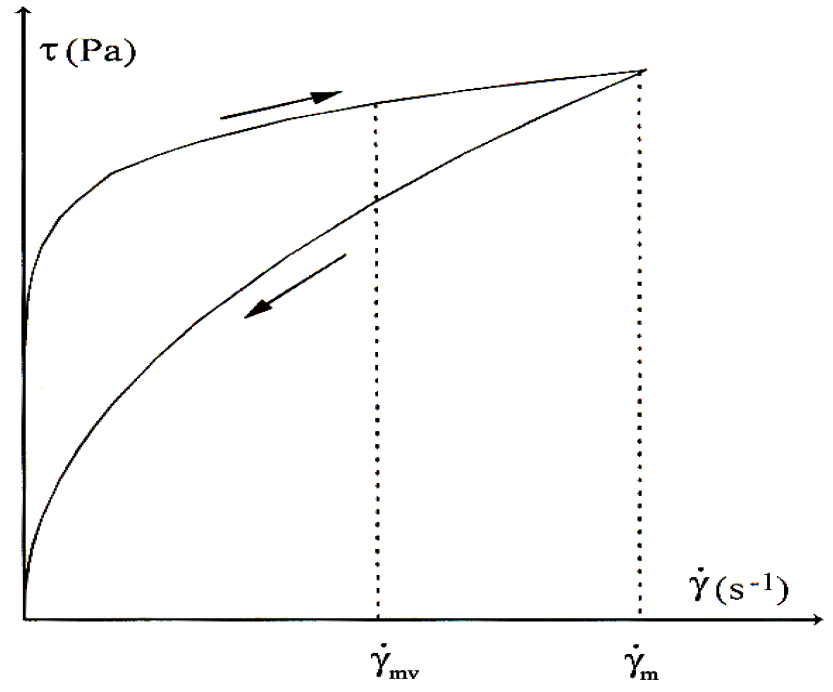
Thixotopic systems, under application of external mechanical forces, loose their internal organization and structure exhibiting thus the decay of the viscosity, by time (Đaković, 1979) which is followed by a gradually recovery of the structure (viscosity) when the force is removed. Thixotropy is usually evaluated by measuring the area enclosed between ascending and descending flow curves obtained by linearly increasing and decreasing shear rate over time. This test is named hysteresis loop test and was developed by Green and Weltmann (1946). Fig. 1 shows one typical hysteresis loop.
The value of the hysteresis loop area indicates the energy required to break down the thixotropic structure (Schramm, 2000). Although useful for demonstrating the thixotropic behaviour of different product the hysteresis area is considered to be the qualitative measure of thixotropy since it depends on the parameters that define hysteresis loop method: the maximum shear rate and the times of duration of linear increasing and decreasing of shear rate (Armelin et al., 2006). Dolz et al. (1997) made an attempt to quantify the hysteresis test by introducing the relative hysteresis area which was defined as the ratio of the hysteresis area to the area beneath the ascending shear curve. Dokić et al. (1999) used the same parameter, but they named it the coefficient of thixotropic breakdown:
 (1)
(1)where:  is the flow equation corresponding to ascending flow curve,
  is the flow equation corresponding to descending flow curve and
  is the maximal shear rate. This coefficient can be calculated by simple integration method. However, in practical rheological measurements maximal shear rate of the rheometer
  (Fig. 1) is usually smaller than the rate
  needed for an instantneous structure breakdown. Dokić et al. (1999) proposed the solution for overcoming the mentioned discrepancy. At
  they applied constant
  for the period of time required for completely breakdown of the structure. That way a truncated thixotropic loop was obtained. However, by modeling the flow curves with different equations they succeeded to predict the maximal shear rate,
  and to derive the mathematical expression for coefficient of thixotropy that will be dependent only on the parameters of flow equation, and not on the
  .
.
The aim of this article was to determine the truncated flow curves of two different thixo-tropic sample and to calculate the values of maximal shear rate,  and parameters of corresponding flow equations using the expressions given by Dokić et al. (1999) and appropriate software package for numerical analysis. While for the sample having nonideal flow curve it was not possible to calculate
 , the new function was introduced and new solution proposed.
2. Theoretical background
The ascending and descending flow curves in hysteresis loop can be described using various equations. For the purpose of this paper the two most common flow equations were used. The first one was:
where:  is the yield stress and m is the degree of non-Newtonian behaviour. By replacing
  and
and  in the expression (1) with their respective equation (2), the following relation for coefficient of thixotropic breakdown is obtained:
 (3)
(3) where:  ,
,  are yield stresses and m' and m" are parameters of equations corresponding to ascending and descending flow curves.
When the system of flow equations:
is solved for the following conditions:  and
and  , the value of
  is obtained:
 (4)
(4)Substituting  in the equation (3) with the expression (4) and taking into account that
  , the following relation for Kd is obtained:
According to the expression (5), the coefficient of thixotropic breakdown depends only on the degree of non-Newtonian behavior. That means that it is possible to eliminate the influence of one measuring condition – maximum shear rate,  , by modeling the experimental results with the flow curve equation.
The second flow equation used for modeling the flow behavior of the thixotropic system was the Herschel-Bulkley equation:
where:  is the yield stress, K is the measure of consistency of the system and n is showing the degree of non-Newtonian behaviour.
If the flow equation (6) is applied instead of (2), the following relation for coefficient of thixotropic breakdown is obtained:
 (7)
(7)where: , K' and n' are parameters of equation describing ascending flow curve,
  , K" and n" are parameters of equation corresponding to descending flow curve and
  is maximum shear rate.
Since the shear rate in relation (7) depends only on the structure of thixotropic system and does not depend on maximum shear rate of rheometer ( ), the coefficient Kd also does not depend on measuring conditions.
The nature of the equation (6) does not enable  to be calculated directly from the system of equation
  and
and  as it was possible for the equation (2). To calculate the value of
  from the equation (6) the numerical analysis has to be employed. Firstly, new function was introduced:
The aim was to find the value of  at which the function
  becomes zero, because that value of
  corresponds to
 . In numerical analysis these values of
  are called the roots of the function
 . Root finding is usually an iterative procedure, which starts with an estimate of the root and produces better approximations.The iteration is stopped when the following conditions are fulfilled:
(The smallness of f(x) test)
or (The closeness of successive approximations test)
To start looking for a root, one needs to give the presumption value for a root. This value can be given as interval (bracket way) or as a single number which represent the value close to root (good starting value way). The way of giving the presumption and stopping the iterations depends on the root-finding method used. Some of the root-finding methods are: the Secant method, the Bisection method, the Newton-Raphson method, the False position method etc.
The unknown parameters from both flow equations (Eq. 2 and Eq. 6) were determined by the curve fitting techniques.
MATERIALS AND METHODS
Thixotropic behaviour of two different samples was characterize by hysteresis loop test: shear rate was increased linearly from 0 to 700s-1 in 3 min, held constant at 700s-1 till total system destruction, and decreased linearly from 700 to 0s-1 in 3 min. The flow measurements were performed by HAAKE RheoStress 600 rheometer (Thermo Scientific, Germany) equipped with Z20 cylinder measuring geometry at the temperature of 20±0.1 °C. The numerical analysis was performed using Mathcad Professional 2000 software package.
RESULTS AND DISCUSSION
The experimentally obtained data set for sample 1 is presented in Fig. 2 and Fig. 3, in the form of crosses (×). It can be clearly seen that the maximum shear rate used was not enough for the complete destruction of a sample. For predicting the maximal shear rate, the Eq. 2 was used firstly. The parameters of the model flow equation were calculated using the genfit function. The function has the following form:
where: vx and vy are vectors containing the x-values and the y-values, respectively, of the data, guess is a vector of initial guess values for the parameters and f is the model equation. To get a better fit, f argument is better to be in the form of vector F which first entry is the model equation f, and which remaining entries are the partial derivatives of f with respect to the unknown parameters.
For the Eq. 2 vector F was:
For the Eq. 2 vector F was:

where:  and
and  . Setting the guess vector as guess = (2; 0.5) the following forms of ascending and descending flow equations were obtained:
  and
and  , respectively. They are presented in Fig. 2 as
  and
and  , because of the shortcoming of Mathcad software in writing the functions with dots and accents.
The value of maximum shear rate, calculated using the Eq. 4, was  . Finally the coefficient of thixotropic breakdown, calculated using the Eq. 5 was
  .
.
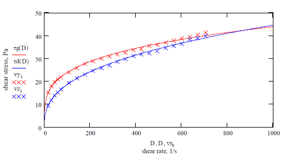 Fig. 2. Flow curve for sample 1 fitted with Equation 2 (experimentally obtained data (×) and theoretically obtained data (___))
The Eq. 6 was also employed for system flow behaviour description. In that case the last argument in genfit function had the following form:

where:  ,
,  and
and  . For guess = (2; 2; 0.5) the following forms of ascending and descending flow equations were obtained:
  and
and  , respectively. They are presented in Fig. 3 as
  and
and  .
.
The maximum shear rate was determined using the root function:
where: f(x) is the function which root is seek, and x is the guess for root value. For our function the root form was:
and obtained value for maximum shear rate was:  s-1. The corresponding coefficient of thixotropic breakdown calculated from the Eq. 7 was:
 .
.
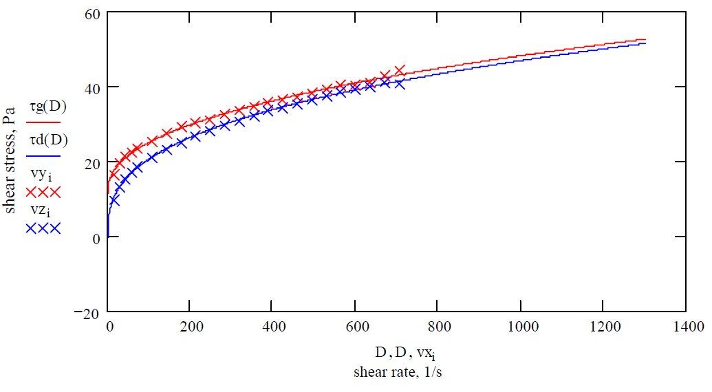
For the sample 2 the same procedure for calculating the maximal shear rate and predicting the maximal shear rate was used. Modeling the experimental data of the sample 2 with the Eq. 2 (Fig. 4) resulted in following ascending and descending flow equation forms, and maximal shear rate and coefficient of thixotropic breakdown values:
However, as it can be seen from the Fig. 5 fitting the experimental data, obtained for sample 2, with the Herschel-Bulkley equation (Eq. 6) did not result in determining the value of maximal shear rate.
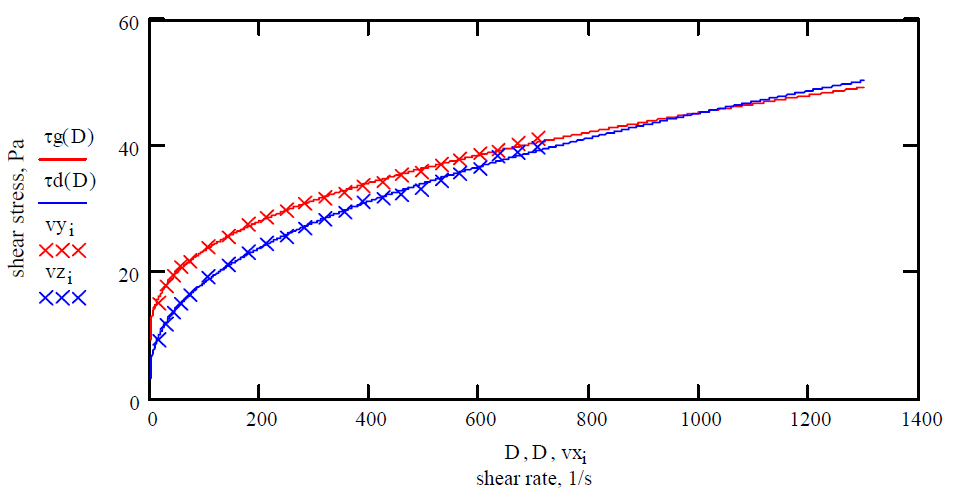 Fig. 3. Flow curve for sample 1 fitted with Equation 6 (experimentally obtained data (×) and theoretically obtained data (___))
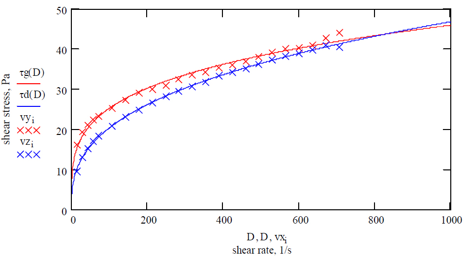 Fig. 4. Flow curve for sample 2 fitted with Equation 2 (experimentally obtained data (×) and theoretically obtained data (___))
The reason was the character of the function 8 (Eq. 8). Namely, the condition for finding the root of the function is that the function is monotonically decreasing. For the real systems it is hardly to achieve since they are of complex nature. Therefore the function 8 was correcting by eliminating the values which disturb the monotonic of the function.
Equation 6 (experimentally obtained data (×) and theoretically obtained data (___))
The function 8 before and after correction is shown in Fig. 6.
The function 8 before and after correction is shown in Fig. 6.
New, corrected results were modeled with the Eq. 6 following the same procedure as for uncorrected results and the obtained values for ascending and descending flow equation forms, and maximal shear rate and coefficient of thixotropic breakdown values were:
All the obtained results are summarized in Table 1. Since, the aim was to approximate the experimental data with the corresponding flow equation, the quality of approximation (correlation) was evaluated by least square (LS) method. The results are listed in Table 1, too.
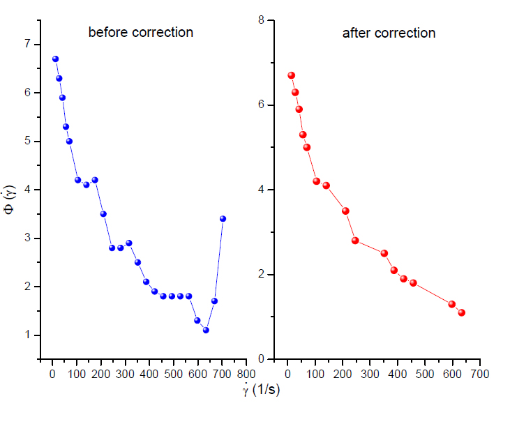 Fig. 6. Function describing the difference between ascending and descending flow curve before and after correction
Table 1. Various parameters and least square values (LS) obtained modeling the samples by different flow equation
|
|
Flow equation |
||
|
Sample |
|
|
|
|
Sample 1 |
Ascending flow curve eq. |
|
|
|
Descending flow curve eq. |
|
|
|
|
LS value for a. curve |
7.0951 |
2.1942 |
|
|
LS value for d. curve |
5.1297 |
4.0172 |
|
|
|
870.24 |
1015 |
|
|
Kd |
0.084 |
0.072 |
|
|
Sample 2 |
Ascending flow curve eq. |
|
|
|
Descending flow curve eq. |
|
|
|
|
LS value for a. curve |
12.8261 |
8.6079 |
|
|
LS value for d. curve |
2.1509 |
2.0861 |
|
|
|
827.86 |
1010 |
|
|
Kd |
0.075 |
0.057 |
|
According to the results obtained by least square method Eq. 6 approximated the experimental results better than the Eq. 2.
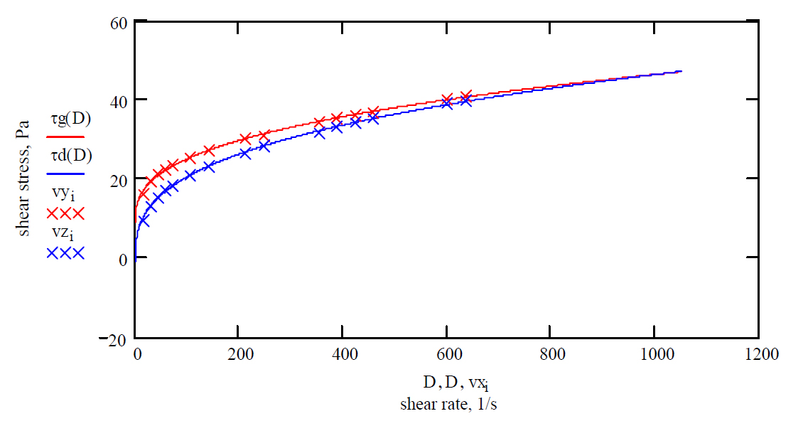 Fig. 7. Corrected flow curve for sample 2 (experimentally obtained data (×) and theoretically obtained data (___))
CONCLUSION
By modeling the experimentally obtained flow curves with different flow equations it is possible to overcome the shortcoming of the rheometers to reach the real maximal shear rate. The same flow equations can also be used to derive the mathematical expressions for the coefficient of thixotropic breakdown. Thus, derived expressions include only the parameters from flow equations, so they are independent on shear rate range used in rheological measurement. However, it is important to choose the appropriate flow equation. The calculations done using Herschel-Bulkley equation were more complicated, because of the nature of the equation. However, this equation better fits to experimentally obtained data which was confirmed by least square calculations.
ACKNOWLEDGMENTS
This work was financially supported by Ministry of Science and Technological Development, Republic of Serbia (project no. 20066)

 JOURNAL TOOLS


 INSTITUTE